Gantt Chart in Google Sheets: How to Create It + Free Templates

A Gantt chart is one of the best project management tools for easy project visualization, planning, and scheduling. In case you’re an avid Google user, read on to learn how to make a Gantt chart in Google Sheets — and get access to our free Gantt chart templates.

How do I make a Gantt Chart in Google Sheets?

The easiest way to create a Gantt chart in Google Sheets is with a stacked bar chart. 

We’ll show you 3 methods you can use to make:

• A basic Gantt chart,
• An advanced Gantt chart with automated progress bars, and
• A manual Gantt chart.

Method #1: Basic Gantt chart

If you need a universal chart that can be used for various projects spanning weeks or months, go for a basic Gantt chart.

To make a basic Gantt chart, you should:

• Make a task table,
• Calculate each task’s start day and duration,
• Create a stacked bar chart,
• Edit the stacked bar chart to look like a Gantt chart, and
• Customize your Gantt chart.

Step #1: Make a task table

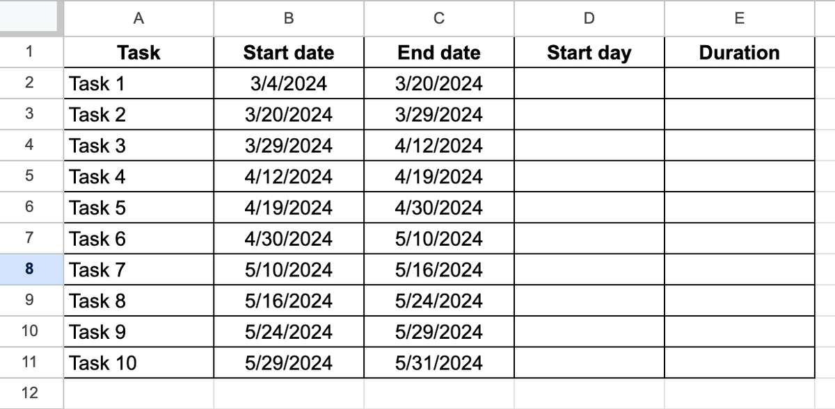
Create a table with 5 different columns in the following formats:

1. Task (text),
2. Start date (date),
3. End date (date),
4. Start day (number), and
5. Duration (number).

Fill out only the first 3 columns with project information. 

Step #2: Calculate each task’s start day and duration

To calculate the first task’s start day, type this formula in cell D2: 

=int(B2)-int($B$2).

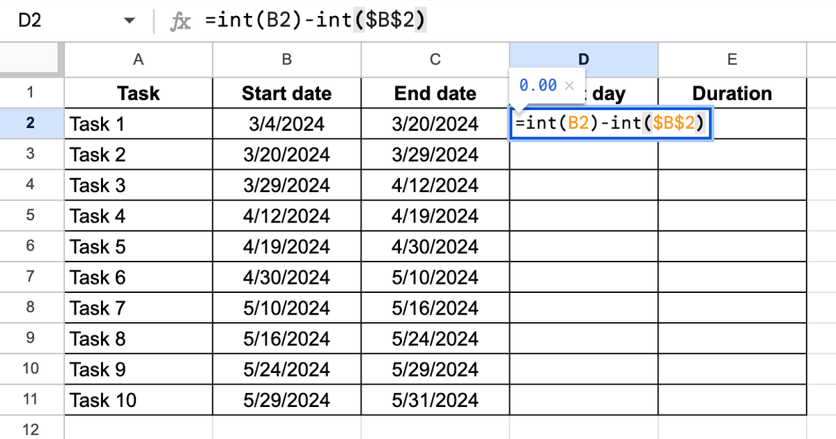
Autofill the column when prompted. 

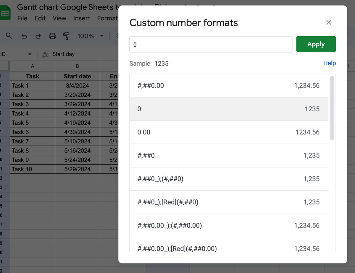
Afterward, change the number format by selecting column D and going to Format > Number > Custom number format. Select the decimal-free version.

To calculate each task’s duration, type this formula in cell E2: 

=C2-B2.

To include a task’s start date in its duration, use this formula instead: 

=INT(C2)-INT(B2)+1.

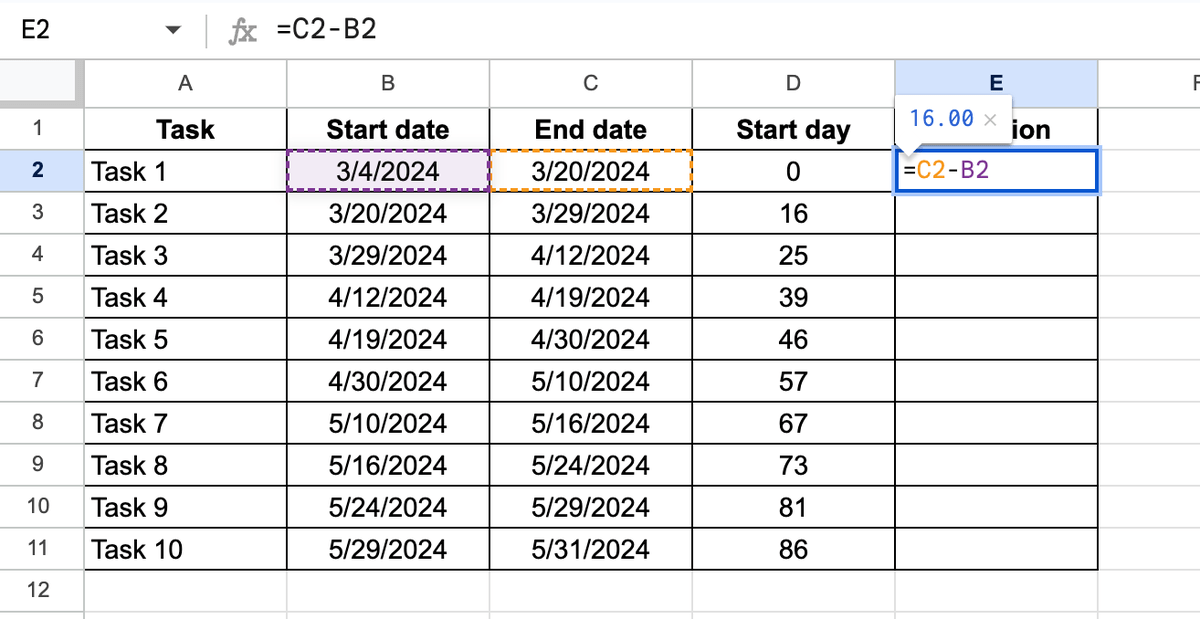
When prompted, autofill the rest of the column and change the number format to a decimal-free version.

Step #3: Create a stacked bar chart

Select the columns you wish to include in your Gantt chart.

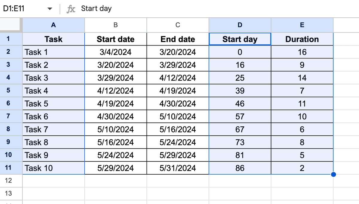
Generate a stacked bar chart by going to Insert > Chart and selecting the stacked bar chart from the Chart type drop-down menu.

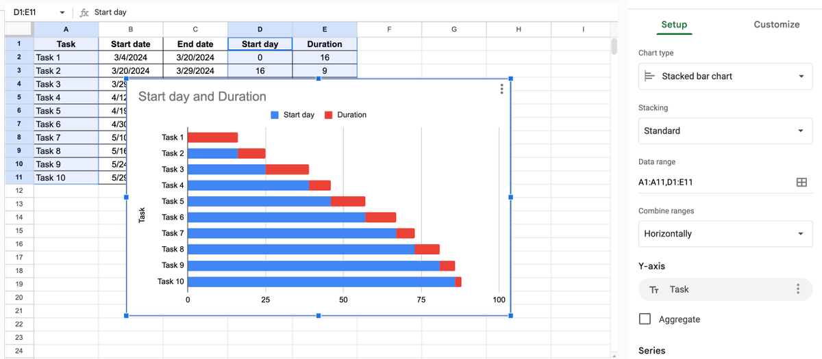
Step #4: Edit the stacked bar chart to look like a Gantt chart

Go to the Series portion of the Chart editor and select Start day from the list.

Once there, change the fill color to white or set the fill capacity to 0% to transform the chart into a Gantt chart.

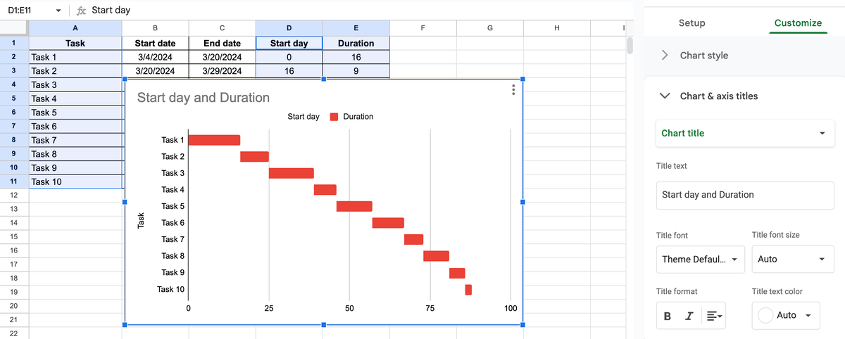
Step #5: Customize your Gantt chart

To customize the chart further, go to the Chart editor > Customize and find the Chart & axis titles section. 

Once there, you can:

• Change the Chart title text to your project title, 
• Omit or change the horizontal and vertical axis titles, and
• Adjust each title’s formatting.

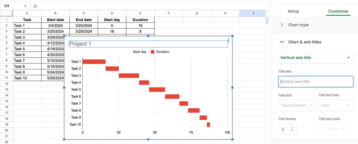
In the Legend section, you can also omit the chart’s legend by choosing None from the list.

What’s more, you can change the project timeline intervals in the Gridlines and ticks section by:

• Choosing the horizontal axis from the list,
• Typing “7” in the Major step field for a weekly chart.

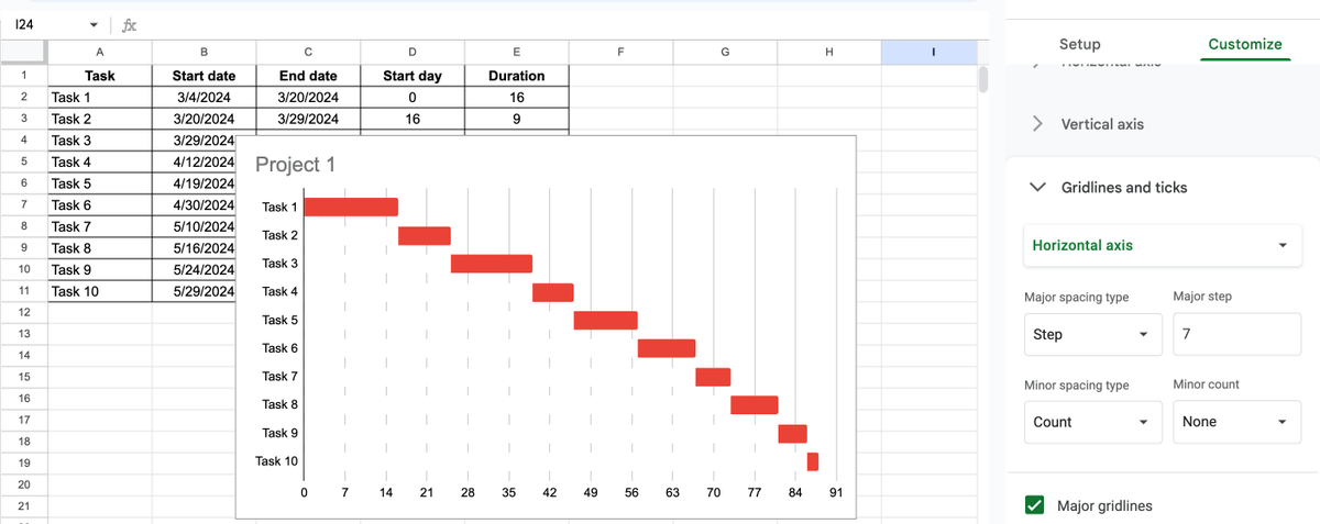
Finally, to customize the chart’s appearance, go to the Chart style section of the Chart editor and choose:

• A new background color,
• Font, and
• A new chart border color.

If you change the background color, remember to change the Start day fill color to the same shade.

In the Series section, you can also change the fill color for the task duration bars.

Alternatively, double-click each bar individually to bring up the Format data point section and pick a different color for each bar.

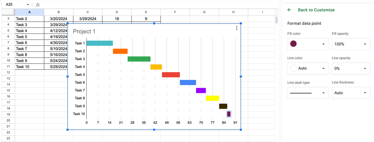
And that’s it! You now have your basic Gantt chart.

Method #2: Advanced Gantt chart

In case you want a more detailed view of your project performance, make an advanced Gantt chart with automated progress bars.

To make an advanced Gantt chart, you have to:

• Calculate when each task starts,
• Make a task progress column,
• Calculate Completed days and Remaining days for each task,
• Create a stacked bar chart, and
• Edit the stacked bar chart to look like a Gantt chart.

Step #1: Calculate when each task starts

This method starts the same as the previous one, so before moving on, make sure you have:

• Created a table and added all the pertinent project details, and
• Calculated task duration.

Like in method #1, calculate each task’s duration with this formula: 

=C2-B2.

If you already know the duration and want to calculate the end dates, use this formula instead: 

=B2+D2.

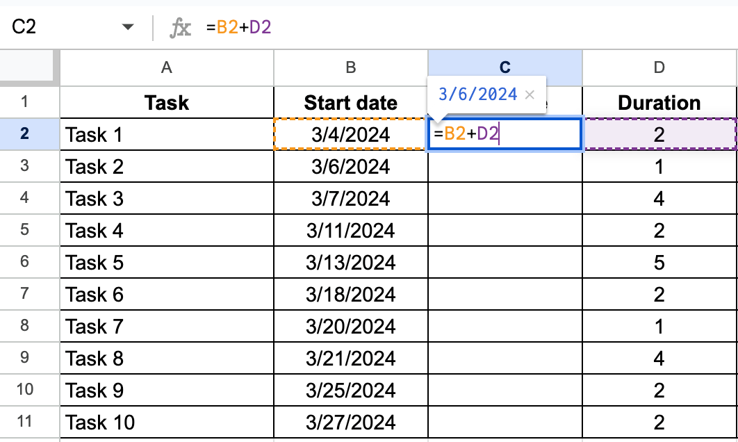
This chart is suitable for month-long projects, so we won’t need the Start day column. 

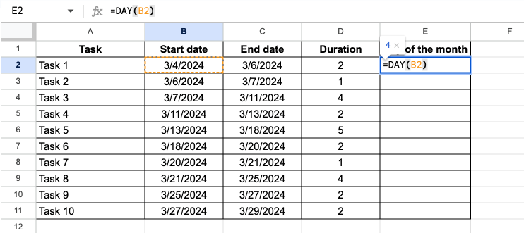
However, we’ll add a Day of the month column (E) next to the Duration column.

To see the day of the month each task starts, use the DAY function in cell E2: 

=DAY(B2). 

Autofill the rest of the column.

Step #2: Make a task progress column

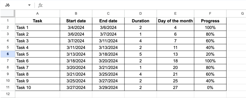
To see the progress of each task, make a Progress column (F). 

Format the column to show percentages by navigating to Format > Number > Custom number format and choosing “0%” from the list.

Now, add the percentage of completed work for each task. 

Step #3: Calculate Completed days and Remaining days for each task

To figure out how many days have been completed for each task, create a new column (G) and use this formula in cell G2: 

=IF((C2)=””,””,(F2*D2)).

Autofill the rest of the column.

To see how many days remain for each task, create a new column (H) and use this formula in cell H2: 

=IF(G2=””,””,(D2-G2)).

Autofill the column when prompted.

Step #4: Create a stacked bar chart

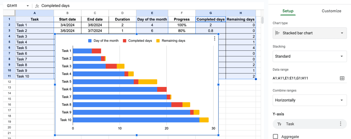
Select columns A, E, G, and H, go to Insert > Chart, and choose the stacked bar chart from the list.

Step #5: Edit the stacked bar chart to look like a Gantt chart

Go to the Chart editor > Customize > Series and pick Day of the month from the list.

Set the fill color to white or change the fill opacity to 0% to make the blue bar disappear.

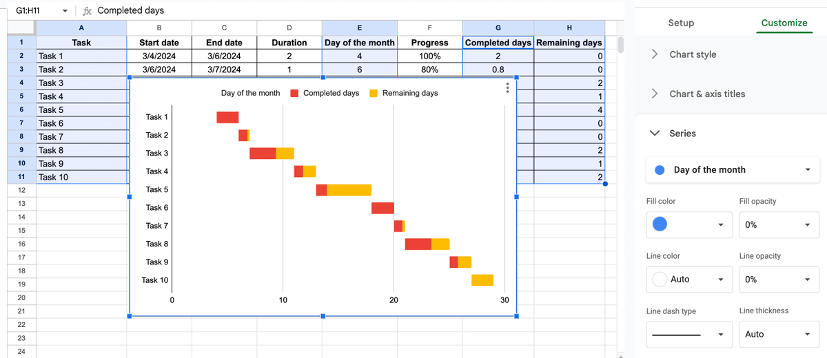
Now, customize the chart further as explained in the previous method by:

• Changing or removing the chart and axis titles,
• Changing the formatting of the vertical and horizontal axis,
• Removing the chart legend,
• Changing the timeline’s intervals, and
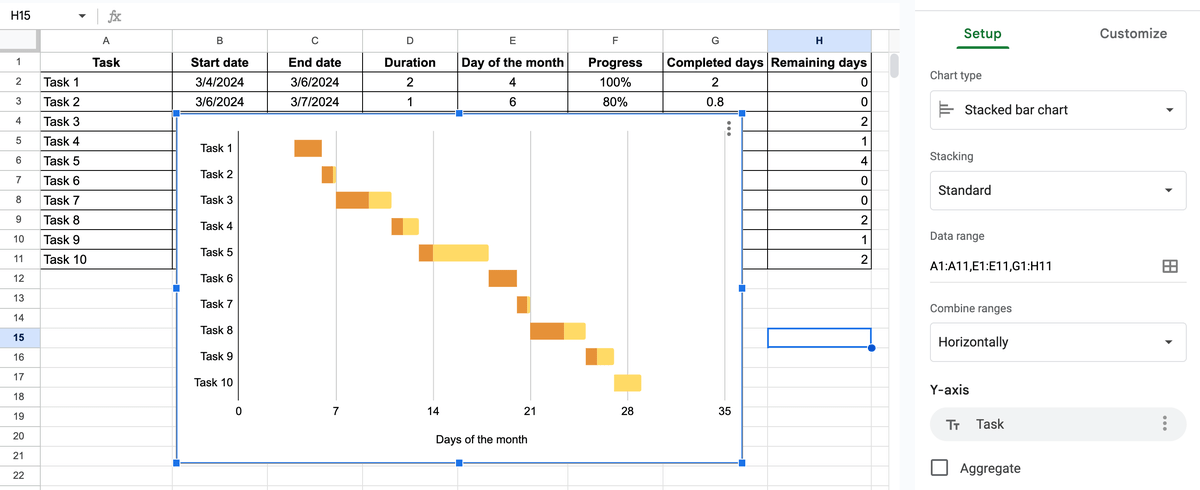
• Customizing the chart’s color scheme and appearance.

Once done, your chart may look something like this.

Method #3: Manual Gantt chart

If stacked bar charts don’t appeal to you, and you want more control over the information included in your Gantt chart, you can also build one from scratch.

To build a manual Gantt chart, you should:

• Make a task table and calculate task duration,
• Format the sequence of days,
• Format the days of the week,
• Use conditional formatting to mark the weekends, and
• Automate the Gantt chart. 

Step #1: Make a task table and calculate task duration

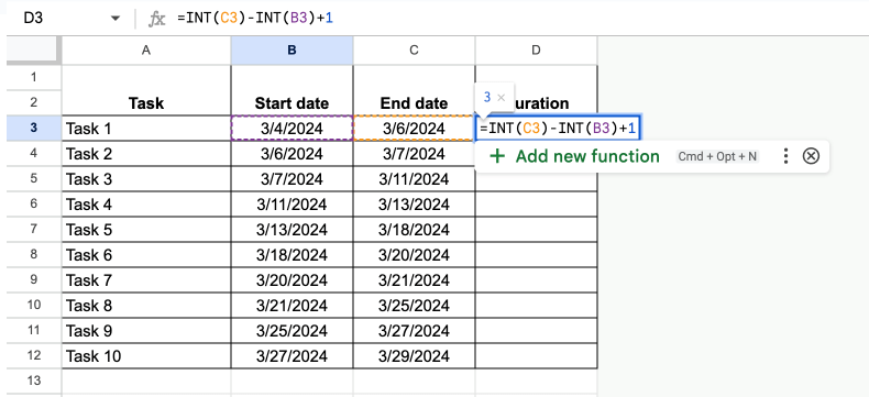
Make a table with 4 columns in the following formats:

• Task (text),
• Start date (date),
• End date (date), and
• Duration (number).

The column titles should consist of 2 cells in total.

To calculate duration, use this formula: 

=INT(C3)-INT(B3)+1. 

For this method, you want to include the start date in each task’s duration.

Step #2: Format the sequence of days

Type this formula in cell E1: 

=EOMONTH(B3,-1)+1.

This formula shows the 1st day of the month given in the Start date column.

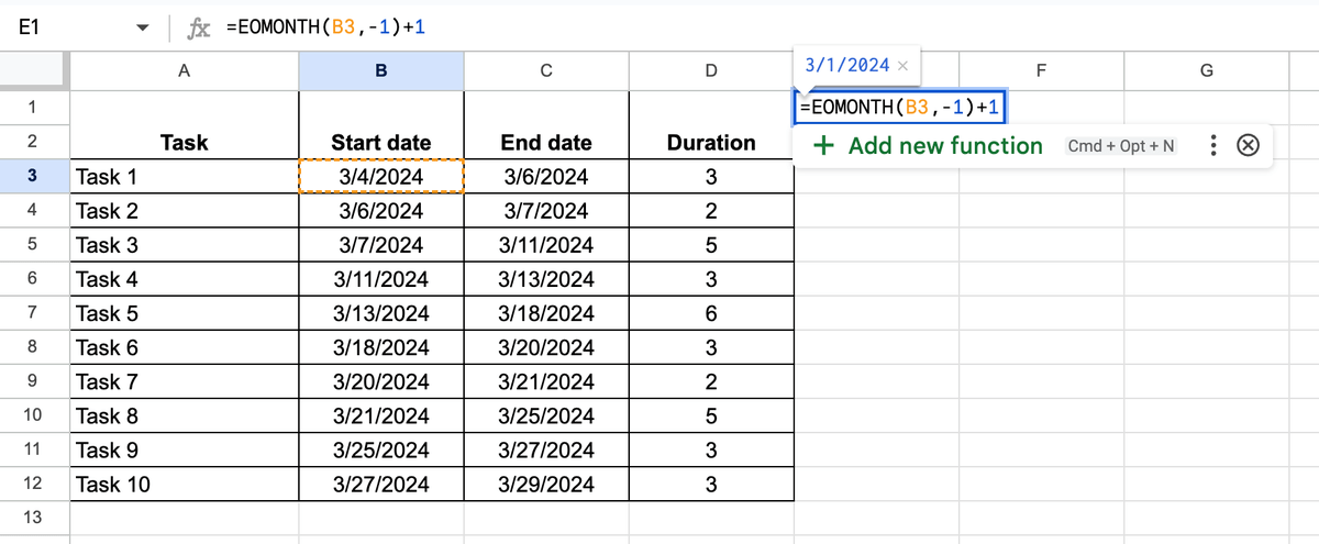
The formula shows the exact date, but you want a single number in this column. 

To get that, select the cell, go to Format > Number > Custom number format, and type “d” in the empty space.

Then, to complete the sequence of days, type this formula in the next cell: 

=E1+1.

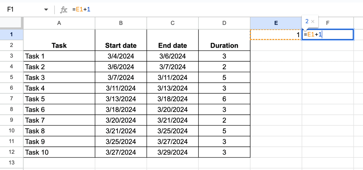
Use the fill handle to copy the formula for the entire month. You may have to add more columns to fit the whole sequence.

Depending on the month you picked, you’ll have 31, 30, or 28/29 columns in total. 

Once done, resize and format the columns.

Step #3: Format the days of the week

To format the cells underneath the sequence of days, use this formula: 

=LEFT(TEXT(E1,”ddd”),1).

The formula will show the 1st letter of the days of the week that correspond to the sequence of days.

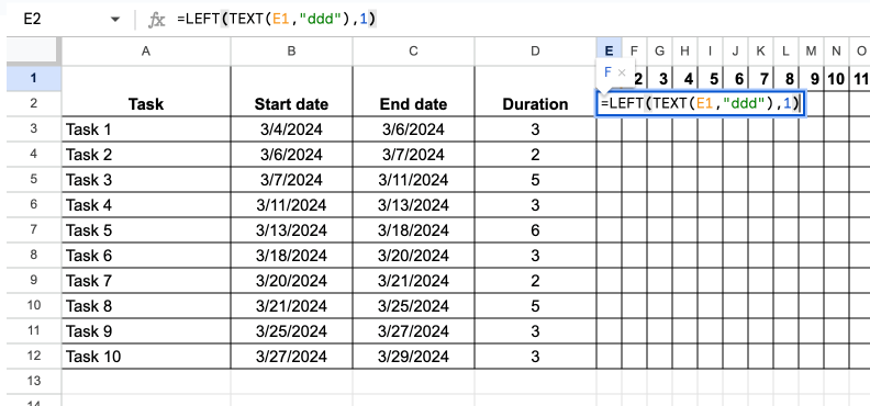
Drag the fill handle to fill out the rest of the columns.

Step #4: Use conditional formatting to mark the weekends

To see which columns are the weekend columns, select the whole Gantt chart area and go to Conditional formatting.

In the Format rules section, select “Custom formula is” from the list and type the following: 

=E$2=”S”.

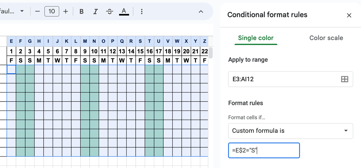
Step #5: Automate the Gantt chart

To automate your Gantt chart, select the same area again and go to Conditional formatting > Add another rule.

Select “Custom formula is” from the list and type the following: 

=AND(E$1>=$B3,E$1<=$C3).

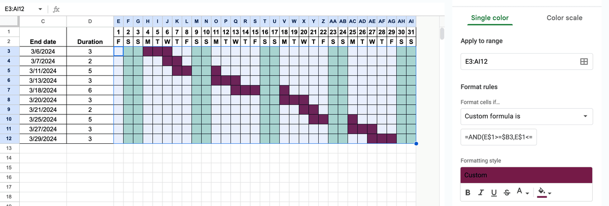
Select another color to distinguish between task duration and the weekend columns. 

If you want to layer the task duration cells over the weekend columns, select the Gantt chart area, go to Conditional formatting, and drag-and-drop the 2nd rule above the 1st one.

Get a free Gantt chart Google Sheets template

If making a Gantt chart from scratch is too much of a hassle, we’ve created a free automated Google Sheets Gantt chart template.

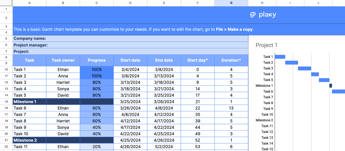
In the document, you’ll find 5 different Gantt chart templates:

• Basic single-project chart,
• Advanced single-project chart,
• Basic multi-project chart, 
• Advanced multi-project chart, and
• Manual Gantt chart.

How to customize your Gantt chart Google Sheets template

Once you’ve copied the template, customize it by:

• Changing the project and task titles,
• Setting task dependencies,
• Using conditional formatting to indicate task progress,
• Changing the progress column’s color scheme, and
• Changing the chart bar colors.

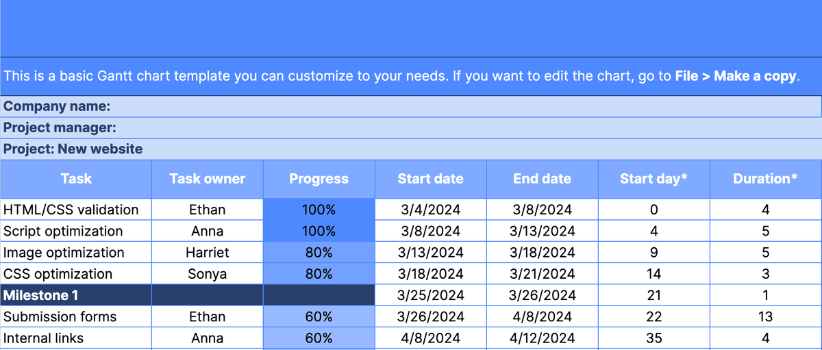
Tip #1: Change the project and task titles

All of the templates have specific areas for typing in the project title.

You can also add your own project tasks and task owners. The changes will be automatically reflected in the Gantt charts.

Tip #2: Set task dependencies

You could simulate the 4 types of task dependencies in Google Sheets with the MAX and MIN functions.

Finish-to-start dependency

A finish-to-start dependency means task B cannot begin until task A has been completed.

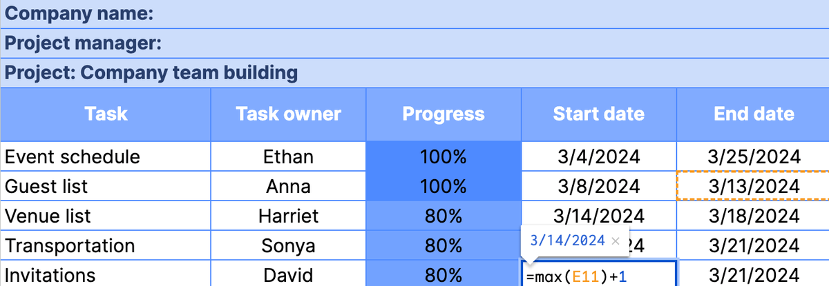
In our example, we have to finish the guest list before making the invitations. So, task A is “Guest list”, while task B is “Invitations.”

To determine task B’s start date, use this formula: 

=MAX(task A end date)+1.

Now, task B starts 1 day after task A ends.

Finish-to-finish dependency

A finish-to-finish dependency means task B cannot be finished until task A has been completed.

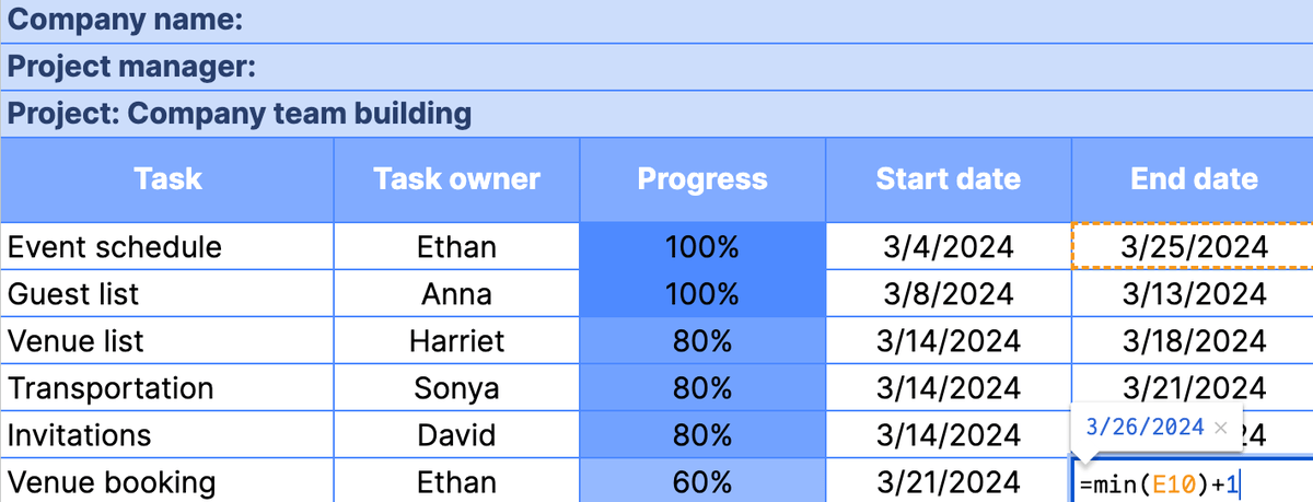
In our example, we need to finish the event schedule (task A) before we finalize the venue booking (task B). 

So, to determine task B’s end date, use this formula: 

=MIN(task A end date)+1.

Now, task B ends 1 day after task A ends.

Start-to-start dependency

A start-to-start dependency means task B cannot start until task A has commenced.

In our example, we cannot start making a list of venues (task B) before we start making the schedule (task A). 

So, to determine task B’s start date, use this formula: 

=MAX(task A start date)+1.

Now, task B starts 1 day after the start of task A.

Start-to-finish dependency 

A start-to-finish dependency means task A has to have started before completing task B.

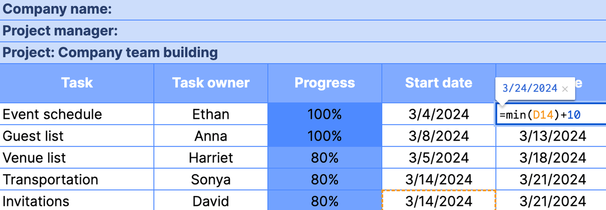
In our example, we must start making invitations (task A) before finalizing the event schedule task (task B).

To determine task B’s end date, use this formula: 

=MIN(task A start date)+10.

Now, task B should be finished 10 days after the initiation of task A.

Tip #3: Use conditional formatting to indicate task progress

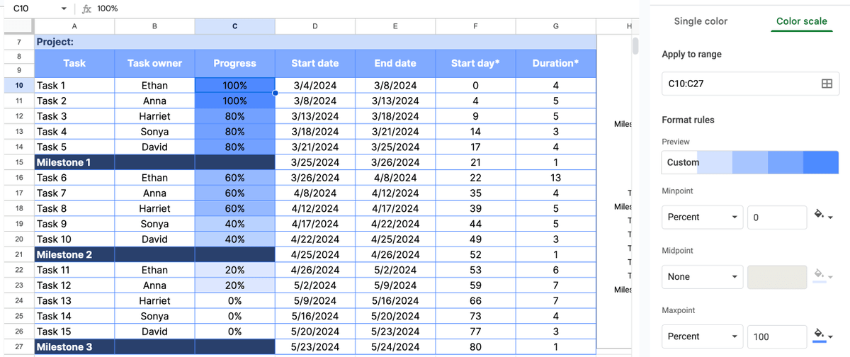
To make Google Sheets automatically graduate colors based on overall task progress, select the progress column and navigate to Format > Conditional formatting.

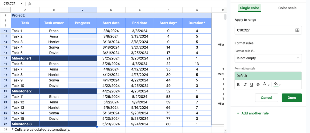
Go to Color scale and select the following:

• For minpoint, choose “Percent” and set the color to white.
• For maxpoint, choose “Percent” and choose any other color.

Google Sheets will then automatically color the cells as you add the percentages.

Tip #4: Change the color scheme

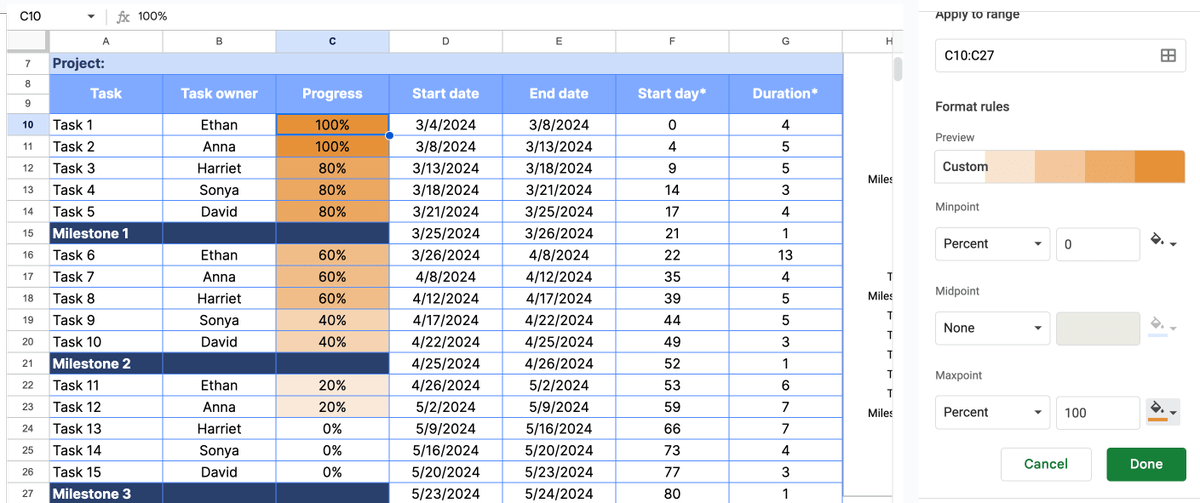
To use another color scheme, select the progress column and navigate to Format > Conditional formatting.

Then, select the pre-set color scale rule and change the maxpoint shade to any other color.

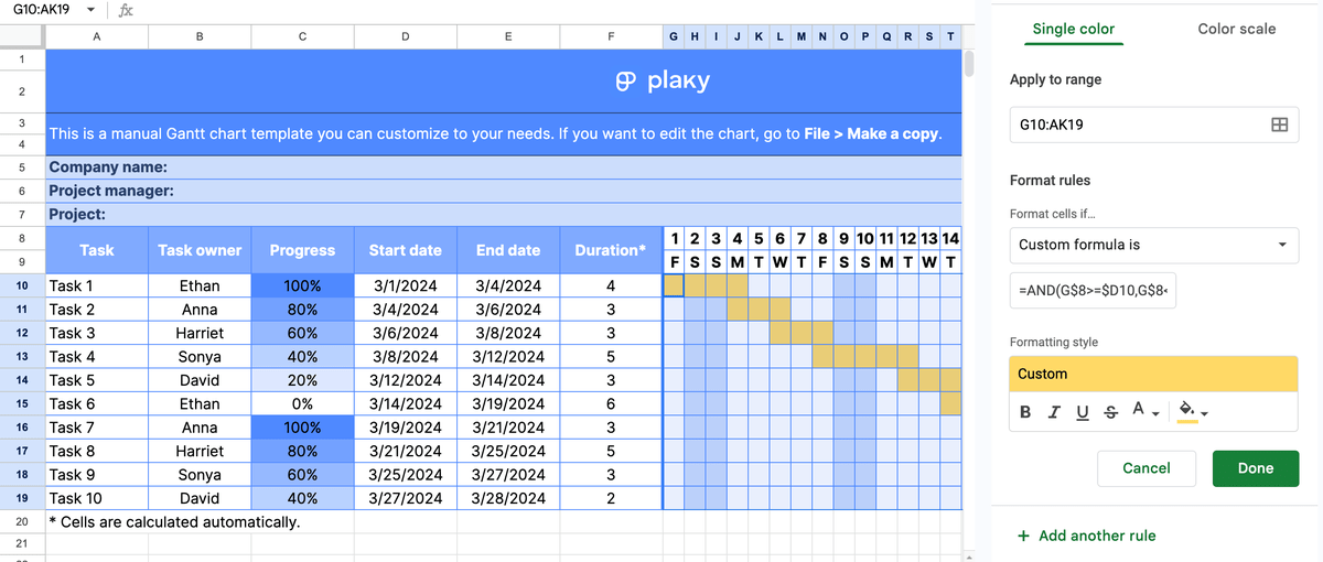
You can also change the color scheme of the whole Gantt area in the manual chart.

Select everything from cell G10 to AK19 and go to Format > Conditional formatting.

Since there are 2 rules set for this area, select the one you want to change and pick another color in the Single color section.

Tip #5: Changing the chart bar colors

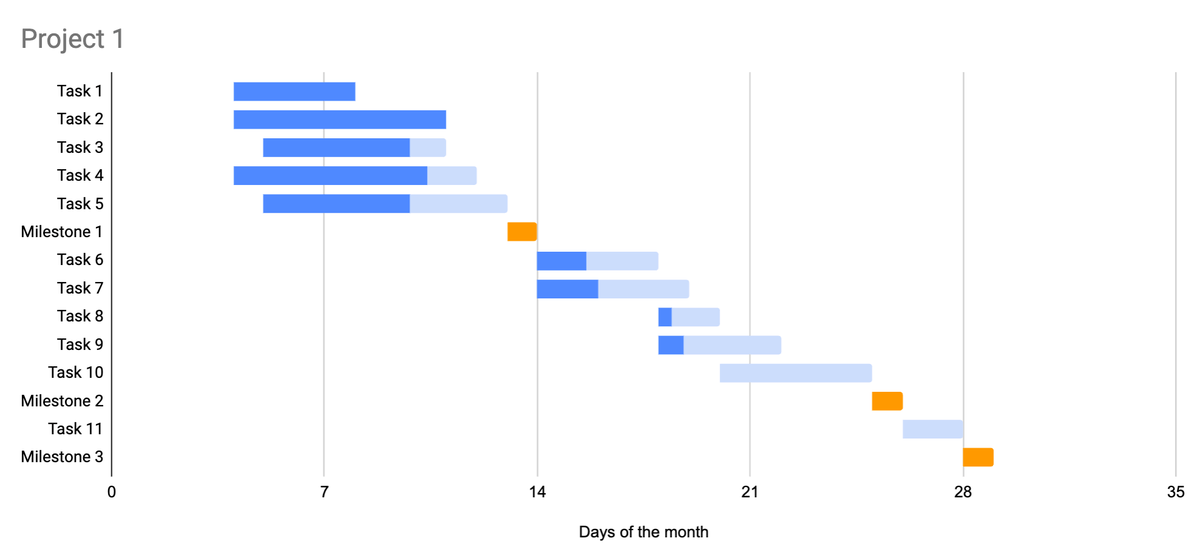
As explained earlier, you can always change your chart’s bar colors. To make the chart easier to read, though, we recommend changing the Milestone bar chart color individually.

Just select each bar and pick another shade in the Chart editor.

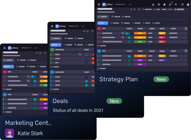
Create a Gantt chart in Plaky

A major downside of making a Gantt chart in Google Sheets is that it takes a lot of time, and it all has to be done manually unless you have a template to rely on.

If you don’t think it’s worth the effort, don’t worry — in Gantt chart software like Plaky, you can make a Gantt chart in 3 easy steps:

• Create a project board,
• Generate a new Gantt view, and
• Customize your Gantt chart.

Step #1: Create a Plaky project board

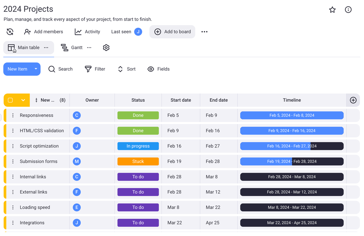
First, create Gantt-compatible fields — Date or Timeline fields. The easiest way to do this is to make a project board and organize your project in the main table first.

Step #2: Generate a new Gantt view

Unlike in Google Sheets, you don’t have to ponder formulas, create and format dozens of columns, or adjust a bar chart to resemble a Gantt chart. 

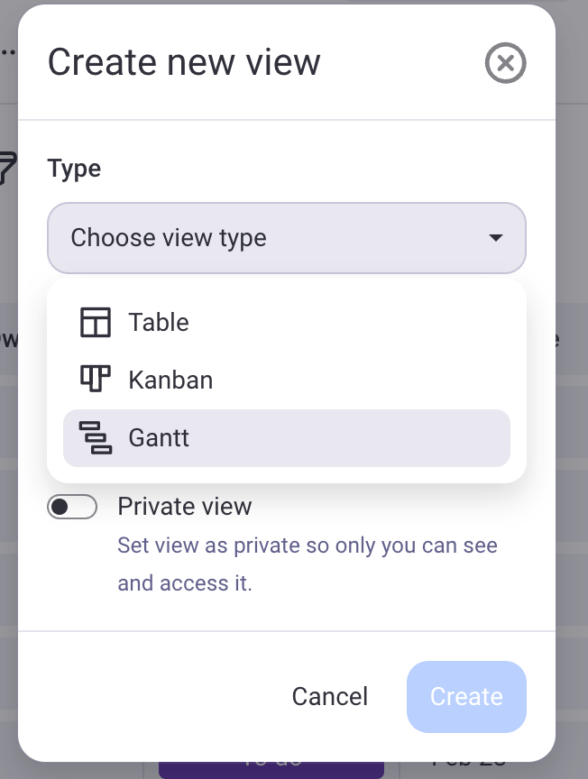
Once you have the main table, create a new view — Gantt. 

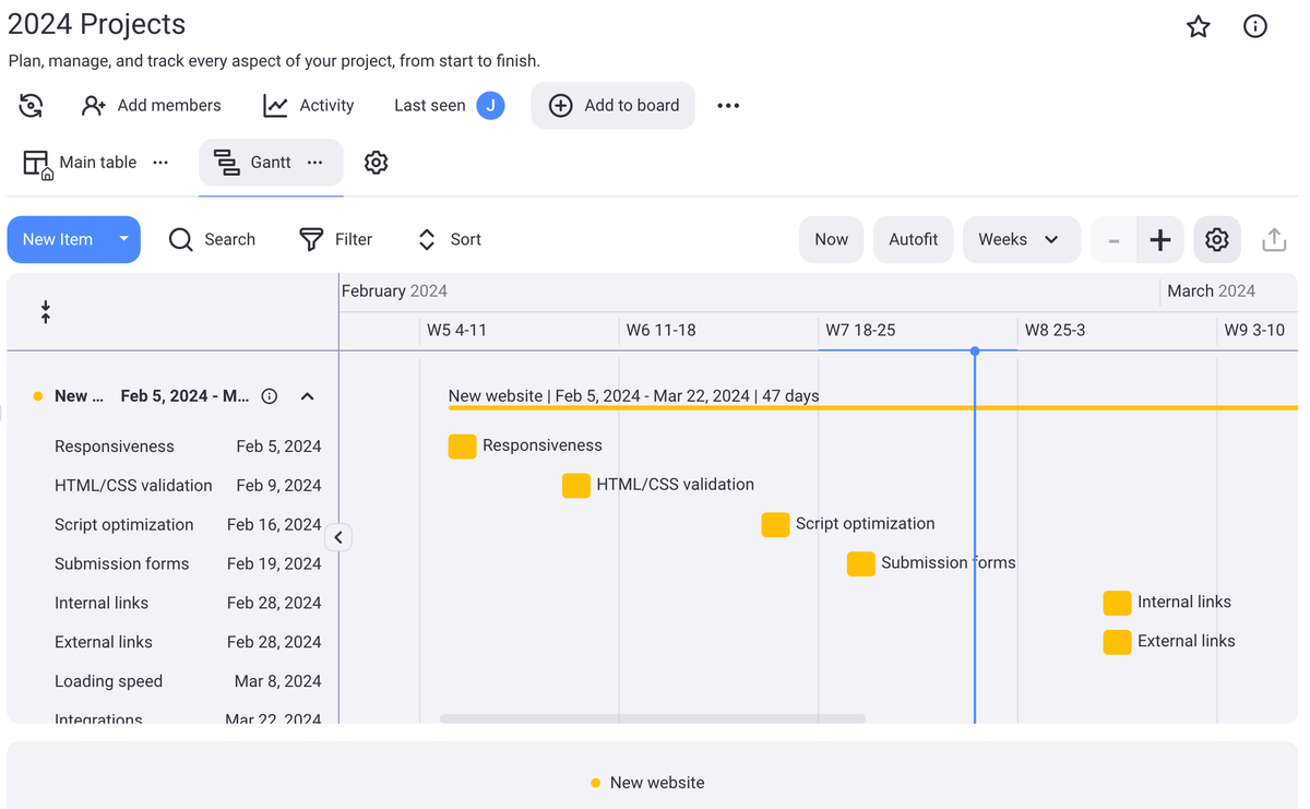
All the information you need for your Gantt chart will be automatically pulled from the main table.

Step #3: Customize your Gantt chart

You can now manipulate the data in the chart by dragging and dropping the tasks wherever you want on the timeline to create a better, more efficient project workflow.

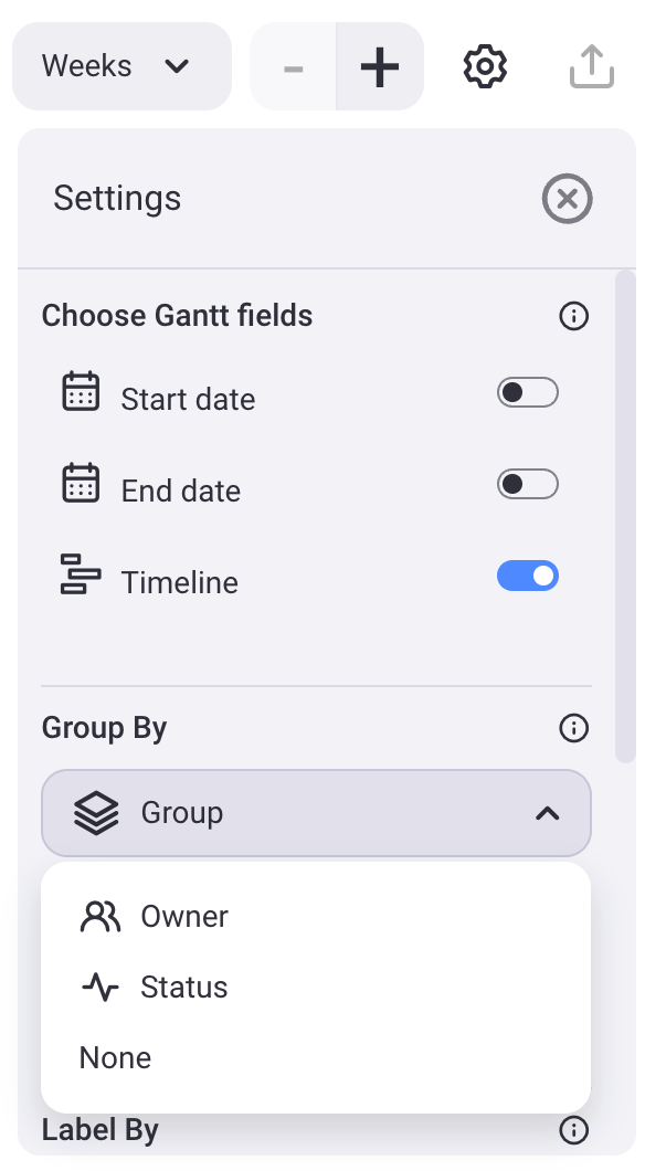
You can also choose how the data should be displayed in the chart in Gantt view settings.

For instance, you can change:

• The fields the chart shows,
• The item grouping criteria,
• The task labeling criteria, and
• The task coloring criteria.

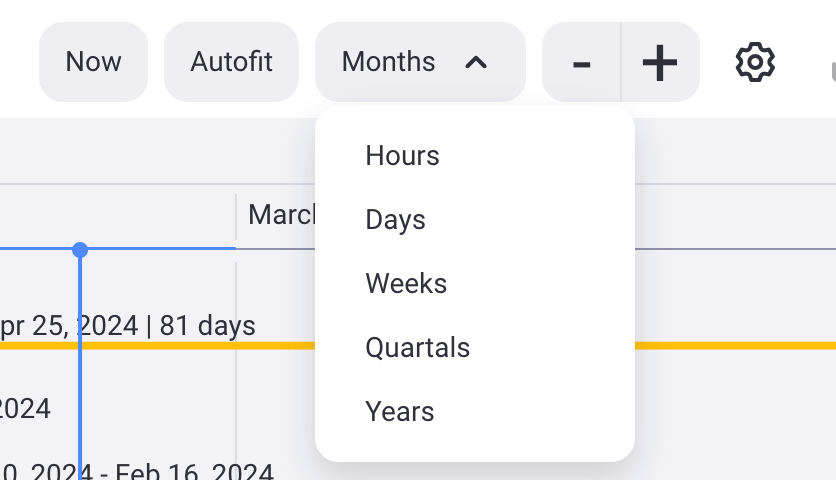
Unlike Google Sheets, Plaky lets you easily toggle between different time periods, depending on the data you want to see. 

What’s more, you can use the Now button when you want to focus on today’s date, and Autofit to fit the task timelines into view.

Google Sheets Gantt chart FAQ

Let’s go through some of the most commonly asked questions about making a Gantt chart in Google Sheets.

Does Google Sheets have a Gantt chart template?

Google Sheets has Smartsheet’s Gantt chart template in its project management category. 

The template resembles our manual Gantt chart template, but since it’s not automated, you’d have to fill it out manually.

Does Google Sheets have a Gantt chart tool?

Google Sheets doesn’t have a specific Gantt chart tool, but as of recently, certain workspace users can get similar results with the Google Sheets Timeline view.

Can I make a Gantt chart template in Google Sheets?

You can build your Gantt chart template from scratch and save it for future use. 

When you want to use the template for another project, open the file, go to File > Make a copy, and then edit that sheet accordingly.

How do I format a monthly Gantt chart in Google Sheets?

Instead of typing “7” when changing the chart’s timeline intervals, you can also type “30” to get a monthly Gantt chart.

However, the result won’t be perfect since not all months have 30 days.

Rely on Gantt charts for effective project visualization

When eager to monitor your project’s progress, there’s hardly a better tool to go for than a Gantt chart.

Within Google Sheets, it’s possible to create a few different kinds of Gantt charts to keep a close eye on your project’s development. 

Still, if you’re not familiar with Google Sheets, project management software like Plaky is bound to help you effortlessly generate highly effective Gantt charts.

As the latest addition to Plaky’s repertoire, the Gantt view makes it easier to visualize your entire project workload, providing you with a high-level overview of your project tasks, schedule, and overall progress.

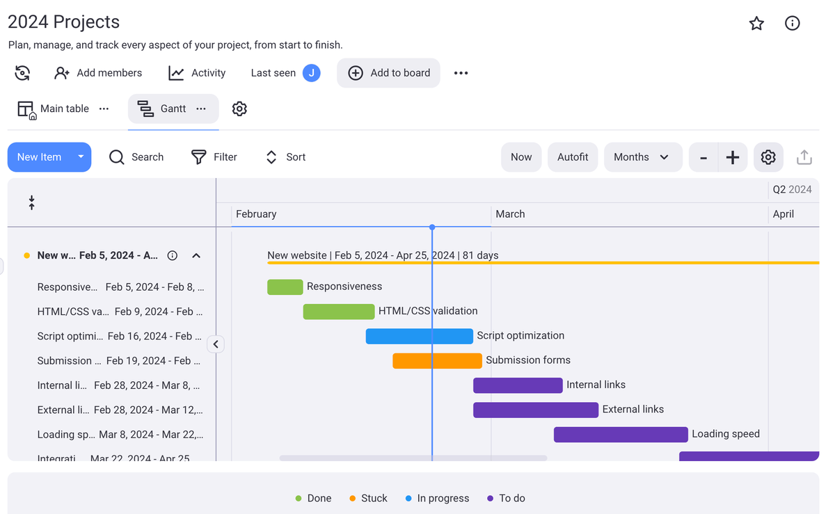
Enjoy a comprehensive overview of all your project tasks and make managing projects and meeting deadlines practically effortless with Plaky’s Gantt charts. Sign up for a free Plaky account today.